BSET Tutorial

Introduction

BSET (Bayesian Surrogate Evaluation Test) is an R package for assessing the validity of surrogate markers in clinical trials. It provides hypothesis testing tools to evaluate whether a surrogate can reliably estimate the causal effect of a treatment on a primary outcome. The package implements the imputation-based Bayesian methodology of Carlotti and Parast (2026), extending the frequentist rank-based approach of Parast et al. (2024). BSET addresses key limitations of the frequentist method, including the lack of causal interpretability and the inability to adjust for covariates in the estimation process.

The package supports Bayesian testing both with and without baseline covariates. Additionally, it includes comprehensive simulation suites to replicate studies from both papers, enabling performance comparisons between Bayesian and frequentist approaches across diverse clinical scenarios.

Installation

The package is not yet available on CRAN, but you can install the development version of BSET from GitHub with:

# install.packages("pak")
# pak::pak("PietroCarlotti/BSET")

To follow along with the examples in this tutorial, you will also need to install the following packages:

library(ggplot2)
library(dplyr)

Quick Start

This section provides a minimal working example for readers who want to apply BSET to their data right away. The main function is BSET, which runs the test with or without adjusting for covariates depending on whether the X argument is provided. It requires a data frame with columns for the primary outcome Y, the surrogate S, and the treatment assignment Z. When X is provided, the model additionally adjusts for those baseline covariates.

To illustrate the usage of the package, we simulate a small dataset with a binary covariate:

# Set the random seed for reproducibility
set.seed(1234)

# Sample size
n <- 50

# Binary covariate
X <- rbinom(n, 1, 0.5)

# Treatment assignment
Z <- rbinom(n, 1, 0.5)

# Primary outcome
Y <- 2 * Z -3 * X + rnorm(n)

# Surrogate outcome
S <- Y + rnorm(n)

df <- data.frame(
  Y = Y,
  S = S,
  Z = Z,
  X = X
)

To run BSET without adjusting for covariates, pass the data frame and the names of the relevant columns:

result_no_X <- BSET::BSET(
  data = df,
  Y = "Y",
  S = "S",
  Z = "Z",
  seed = 123,
  plot = TRUE
)
result_no_X$theta_posterior_plot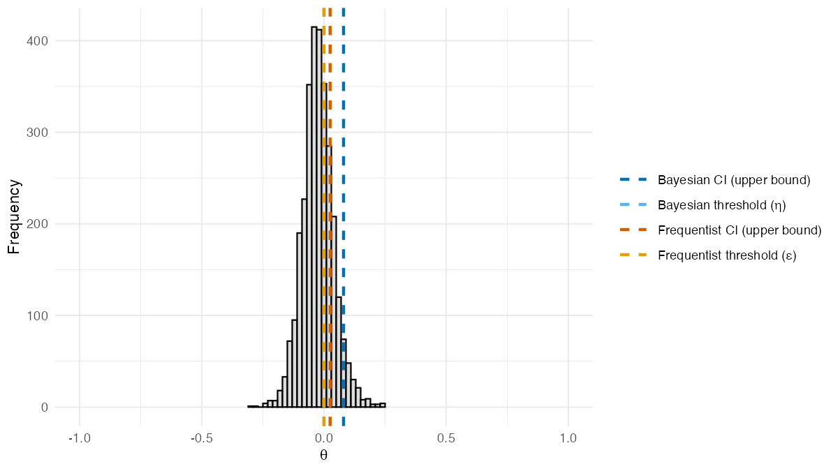

$Posterior distribution of $\theta$ from `BSET` without covariates. Dashed lines show estimated quantities: the Bayesian 95\% credible interval upper bound and threshold $\eta$ (blue shades), and the frequentist 95\% confidence interval upper bound and threshold $\varepsilon$ (orange shades).$

Posterior distribution of $\theta$ from BSET without covariates. Dashed lines show estimated quantities: the Bayesian 95% credible interval upper bound and threshold $\eta$ (blue shades), and the frequentist 95% confidence interval upper bound and threshold $\varepsilon$ (orange shades).

To run BSET with a baseline covariate, add the covariate column name via the X argument:

result_X <- BSET::BSET(
  data = df,
  Y = "Y",
  S = "S",
  Z = "Z",
  X = "X",
  seed = 123,
  plot = TRUE
)
result_X$theta_posterior_plot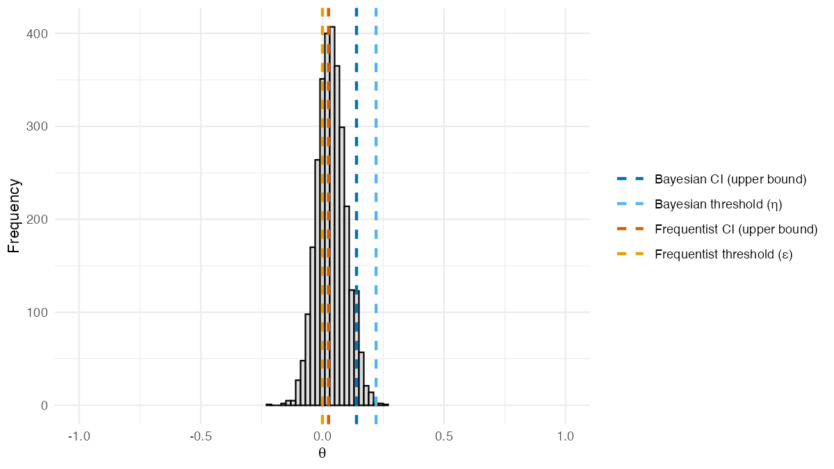

$Posterior distribution of $\theta$ from `BSET`, adjusted for a baseline covariate. Dashed lines show estimated quantities: the Bayesian 95\% credible interval upper bound and threshold $\eta$ (blue shades), and the frequentist 95\% confidence interval upper bound and threshold $\varepsilon$ (orange shades).$

Posterior distribution of $\theta$ from BSET, adjusted for a baseline covariate. Dashed lines show estimated quantities: the Bayesian 95% credible interval upper bound and threshold $\eta$ (blue shades), and the frequentist 95% confidence interval upper bound and threshold $\varepsilon$ (orange shades).

The function returns the posterior distribution of $\theta$ , the discrepancy between the treatment effects on $Y$ and $S$ . Dashed lines in blue shades mark estimated Bayesian quantities: the upper bound of the 95% credible interval and the validation threshold $\eta$ . Dashed lines in orange shades mark estimated frequentist quantities: the upper bound of the 95% confidence interval and the threshold $\varepsilon$ from Parast et al. (2024). Solid lines mark the true values: purple for $\theta$ and pink for $\delta$ . If the Bayesian credible interval upper bound falls below the threshold $\eta$ , there is evidence that the surrogate is valid.

The rest of this tutorial explains how the data are generated, how the estimands $\delta$ and $\theta$ are computed, and how the validation threshold $\eta$ is calibrated.

Generating the data

We start by setting the random seed for reproducibility of the results.

# Set the random seed for reproducibility
set.seed(1234)

# Sample size and treatment assignment probability used throughout
n <- 50
p <- 0.5

The package includes two functions to generate data for the simulations: DGP and DGP_X. The first one generates data from the simulation settings of Parast et al. (2024), which do not include covariates; the second one generates data which depends on a binary covariate $X$ and is used for the simulations of Carlotti and Parast (2026).

For example, this is how we can generate data from the second setting defined in Parast et al. (2024) (i.e.: the setting where the surrogate is perfect and covariates are not included):

# Mean vector of potential outcomes for the primary outcome and the surrogate
mu_star <- c(6, 6, 2.5, 2.5)

# Covariance matrix of potential outcomes for the primary outcome and the surrogate
Sigma_star <- kronecker(
  diag(2),
  matrix(
    data = c(3, 3,
             3, 3.1),
    nrow = 2,
    ncol = 2)
)

# Generate the data
data_no_X <- BSET::DGP_no_X(
  n = n,
  p = p,
  mu_star = mu_star,
  Sigma_star = Sigma_star,
  model = "Gaussian"
)

While this is how we can generate data from the first setting defined in Carlotti and Parast (2026) (i.e.: the setting where the surrogate is useful and covariates are included):

# Binary covariate probability
q <- 0.5

# Mean vector for potential outcomes when X = 0 and when X = 1
mu_0 <- c(5, 5, 0, 0)
mu_1 <- c(5, -5, 0, -10)

# Covariance matrix for potential outcomes when X = 0 and when X = 1
Sigma_0 <- kronecker(
  diag(2),
  matrix(
    data = c(1, 1,
             1, 2),
    nrow = 2,
    ncol = 2)
  )

Sigma_1 <- kronecker(
  diag(2),
  matrix(
    data = c(1, 1,
             1, 2),
    nrow = 2,
    ncol = 2)
  )

# Generate the data
data_X <- BSET::DGP_X_binary(
  n = n,
  p = p,
  q = q,
  mu_0 = mu_0,
  mu_1 = mu_1,
  Sigma_0 = Sigma_0,
  Sigma_1 = Sigma_1
  )

Computing the true values of the discrepancy parameters

Given the data generated with the above functions, we can estimate $\delta$ and $\theta$ using the compute_delta and compute_theta functions, respectively.

For example, for the data generated without covariates:

# Compute delta
delta_no_X <- BSET::compute_delta(MC_data = data_no_X)

# Compute theta
theta_no_X <- BSET::compute_theta(MC_data = data_no_X)

And for the data generated with covariates:

# Compute delta
delta_X <- BSET::compute_delta(MC_data = data_X)

# Compute theta
theta_X <- BSET::compute_theta(MC_data = data_X)

The estimated values of $\delta$ and $\theta$ are shown in the table below.

Estimated values of $\delta$ and $\theta$ in the two settings.
Setting	$\widehat{\delta}$	$\widehat{\theta}$
No X (Perfect Surrogate)	0.010	0
Binary X	0.212	0

To determine the values of $\delta$ and $\theta$ for all the settings defined in the two papers, we use a large-scale Monte Carlo simulation via the compute_estimands_Parast_et_al_2024 function for data without covariates (Parast et al. 2024), and the compute_estimands_Carlotti_and_Parast_2026 function for data including covariates (Carlotti and Parast 2026). These functions run a Monte Carlo simulation with a large number of samples (e.g., 1,000,000) and can be called as follows:

# Compute Monte Carlo estimands (based on 1,000,000 samples) — this is slow
estimands_Parast_et_al_2024 <- BSET::compute_estimands_Parast_et_al_2024(n_MC = 1000000)
estimands_Carlotti_and_Parast_2026 <- BSET::compute_estimands_Carlotti_and_Parast_2026(n_MC = 1000000)

For the purpose of this tutorial, we load the precomputed versions shipped with the package:

# Load precomputed Monte Carlo estimands (based on 1,000,000 samples)
estimands_Parast_et_al_2024 <- BSET::estimands_Parast_et_al_2024
estimands_Carlotti_and_Parast_2026 <- BSET::estimands_Carlotti_and_Parast_2026

As shown in the table below, $\delta$ and $\theta$ yield identical values (up to Monte Carlo error) across all settings. Both estimands are close to $0$ for a perfect surrogate, they are significantly higher for a useless surrogate, and take intermediate values for imperfect surrogates or misspecified models.

Monte Carlo estimates of $\delta$ and $\theta$ for the simulation settings considered in Parast et al. (2024).
Setting	$\delta$	$\theta$
Useless surrogate	0.293	0.293
Perfect surrogate	0.003	0.003
Imperfect surrogate	0.111	0.111
Misspecified model	0.148	0.148

Whereas, as shown in the table below, when we include covariates in the data generating process, $\delta$ and $\theta$ yield different values. In particular, while $\theta$ is close to $0$ for a perfect surrogate, $\delta$ is significantly higher.

Monte Carlo estimates of $\delta$ and $\theta$ for the simulation settings considered in Carlotti and Parast (2026).
Setting	$\delta$	$\theta$
Perfect surrogate	0.252	0.006
Perfect surrogate	0.357	0.000

Computing the validation threshold

The validation threshold $\eta$ is the value of $\theta$ below which the surrogate is considered valid. As explained in Carlotti and Parast (2026), the computation of $\eta$ is based on the distribution of the following Bayes factor: $BF_{n} = \frac{1 - F_{\text{Beta} \left( a + n \hat{V}_{S}, \, b + n - n \hat{V}_{S} \right)} \left( \frac{1}{2} \right)}{1 - F_{\text{Beta} \left( a, \, b \right)} \left( \frac{1}{2} \right)}.$ Given the true value of $V_S$ , the distribution of $BF_n$ can be computed with the function compute_BF_distribution. For example, the distribution of the Bayes factor under the null hypothesis $V_S = 0.5$ can be computed as follows:

# Hypothesized value of V_S under the null
V_S_zero <- 0.5

# Prior parameters for the Beta distribution
a <- 1
b <- 1

# Alternative hypothesis for the Bayes factor
BF_alternative <- "greater"

# Compute the distribution of the Bayes factor
BF_distribution <- BSET::compute_BF_distribution(
  n = n,
  V_S_true = V_S_zero,
  V_S_zero = V_S_zero,
  a = a,
  b = b,
  BF_alternative = BF_alternative
)

The distribution of the Bayes factor under the null hypothesis is shown in the figure below. Since the Bayes factor can take values on a very wide range, we plot the distribution on the log scale.

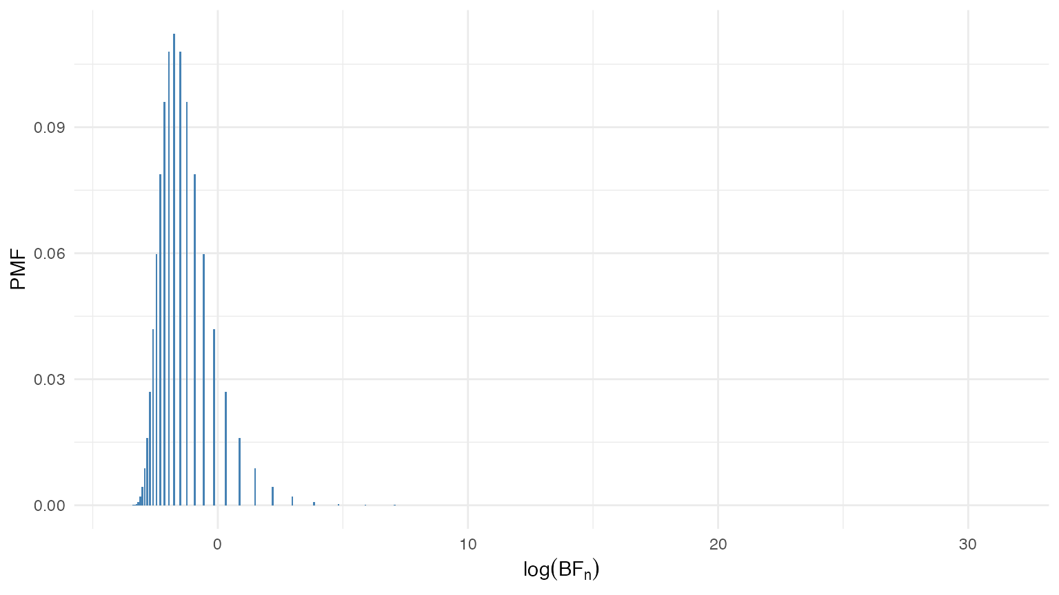
Distribution of the Bayes factor under the null hypothesis $V_S = 0.5$ .

Given the distribution of the Bayes factor under the null hypothesis, we can compute the critical value $BF_{n, \alpha}$ corresponding to a specified Type I error rate $\alpha$ .

# Type I error rate
alpha <- 0.05

# Compute the critical value of the Bayes factor corresponding to alpha
BF_alpha <- BF_distribution %>%
    dplyr::filter(BF_CDF >= 1 - alpha) %>%
    dplyr::slice(1) %>%
    dplyr::pull(BF_values)

For example, for $\alpha = 0.05$ we have

$BF_{n, \alpha} = 1.385.$

Once we have the value of $BF_{n, \alpha}$ , we can compute the value of $v_S$ that satisfies the following equation:

$P(\text{BF}_n \geq \text{BF}_{n, \alpha} \; | \; V_S = v_S) = 1 - \beta,$

where $1 - \beta$ is the desired power of the test. A root-finding algorithm is used to solve for the value of $v_S$ that satisfies the above equation, which is implemented in the function compute_V_S_star.

For example, for a Type II error rate of $\beta = 0.2$ , we can compute the value of $v_S$ as follows:

# Type II error rate
beta <- 0.2

# Compute the value of v_S that satisfies the power constraint
V_S_star <- BSET::compute_V_S_star(
  n = n,
  alpha = alpha,
  beta = beta,
  V_S_zero = V_S_zero,
  a = a,
  b = b,
  BF_alternative = BF_alternative,
  root_tolerance = 1e-16
)$V_S_star

Then, we have that

$v_S = 0.685.$

Finally, the validation threshold $\eta$ can be computed as

$\eta = \max \{v_Y - v_S, 0\},$

where $v_Y$ is the hypothesized value of the treatment effect on the primary outcome (typically set equal to the estimate computed on the available data).

For example, we can set $v_Y$ equal to the Monte Carlo estimate of $V_Y$ for setting 1 of Parast et al. (2024) (i.e.: the setting where the surrogate is perfect and covariates are not included).

# Hypothesized value of the treatment effect on the primary outcome
v_Y <- estimands_Parast_et_al_2024$V_Y_MC[2]

# Compute the validation threshold eta
eta <- max(v_Y - V_S_star, 0)

In this case, we have that

$\eta = 0.238.$

Running the BSET procedure

The package includes the function BSET to run the BSET procedure. When the X argument is omitted (or set to NULL), the procedure runs without adjusting for covariates; when X is provided, it adjusts for the specified baseline covariates.

The result of the procedure is summarized by the posterior distribution of $\theta$ and its 95% credible interval. In general, if the upper bound of the credible interval falls below the validation threshold $\eta$ , the BSET procedure concludes that there is evidence that the surrogate is valid. If instead the upper bound exceeds $\eta$ , the procedure does not find sufficient evidence of surrogacy.

BSET with no covariates

As an example, we can run the BSET procedure without adjusting for covariates on the data generated from the second setting of Parast et al. (2024). First of all, we need to prepare the data in the format required by BSET: a data frame with three columns, where the first column contains the observed values of the primary outcome $Y$ , the second column contains the observed values of the surrogate $S$ , and the third column contains the treatment assignment $Z$ .

# Prepare the data for BSET (no covariates)
BSET_no_X_data <- data.frame(
  Y = data_no_X$P_observed[, "Y"],
  S = data_no_X$P_observed[, "S"],
  Z = data_no_X$Z 
)

We also need to define the posterior sampling parameters:

n_chains: The number of MCMC chains to run.
n_iter: The total number of MCMC iterations to run for each chain.
burn_in_ratio: The proportion of MCMC iterations to discard as burn-in.

# Posterior sampling parameters
n_chains <- 2
n_iter <- 2000
burn_in_ratio <- 0.25

Then, we need to define the prior parameters for the distribution of the potential outcomes in our Bayesian model. In particular, we need to specify:

mu_0: A numeric vector of length 4 containing the prior means for the potential outcomes.
Sigma_0: A numeric positive-definite matrix of dimension $4 \times 4$ containing the prior covariance matrix for the potential outcomes.
s: A numeric vector of length 4 containing the prior scale parameters for the potential outcomes.
tau: A numeric scalar containing the prior scale parameter for the correlation matrix of the potential outcomes.

# Prior parameters
mu_0 <- rep(0, 4)
Sigma_0 <- diag(4)
s <- rep(1, 4)
tau <- 1

If the true values of $\delta$ and $\theta$ are known, we can also specify them as input to BSET to check whether they are included in the posterior credible intervals. In this case, we can set $\delta$ and $\theta$ equal to the Monte Carlo estimates for setting 2 of Parast et al. (2024).

We can also specify some additional parameters for the BSET procedure, such as:

seed: An integer scalar to set the random seed for reproducibility of the MCMC sampling process.
plot: A logical scalar indicating whether to plot the posterior distribution of $\theta$ .
mute: A logical scalar indicating whether to suppress the output of the MCMC sampling process.
parallel: A logical scalar indicating whether to run the MCMC sampling process in parallel or sequentially.

Finally, we can run the BSET procedure without adjusting for covariates as follows:

# Run the BSET procedure without adjusting for covariates
BSET_no_X_results <- BSET::BSET(
  data = BSET_no_X_data,
  Y = "Y",
  S = "S",
  Z = "Z",
  delta_true = estimands_Parast_et_al_2024$delta_MC[2],
  theta_true = estimands_Parast_et_al_2024$theta_MC[2],
  seed = 123,
  n_chains = n_chains,
  n_iter = n_iter,
  burn_in_ratio = burn_in_ratio,
  a = a,
  b = b,
  alpha = alpha,
  beta = beta,
  V_S_zero = V_S_zero,
  BF_alternative = BF_alternative,
  root_tolerance = 1e-16,
  mu_0 = mu_0,
  Sigma_0 = Sigma_0,
  s = s,
  tau = tau,
  plot = TRUE,
  mute = TRUE,
  parallel = TRUE
)

The posterior distribution of $\theta$ from the BSET procedure without adjusting for covariates is shown in the figure below.

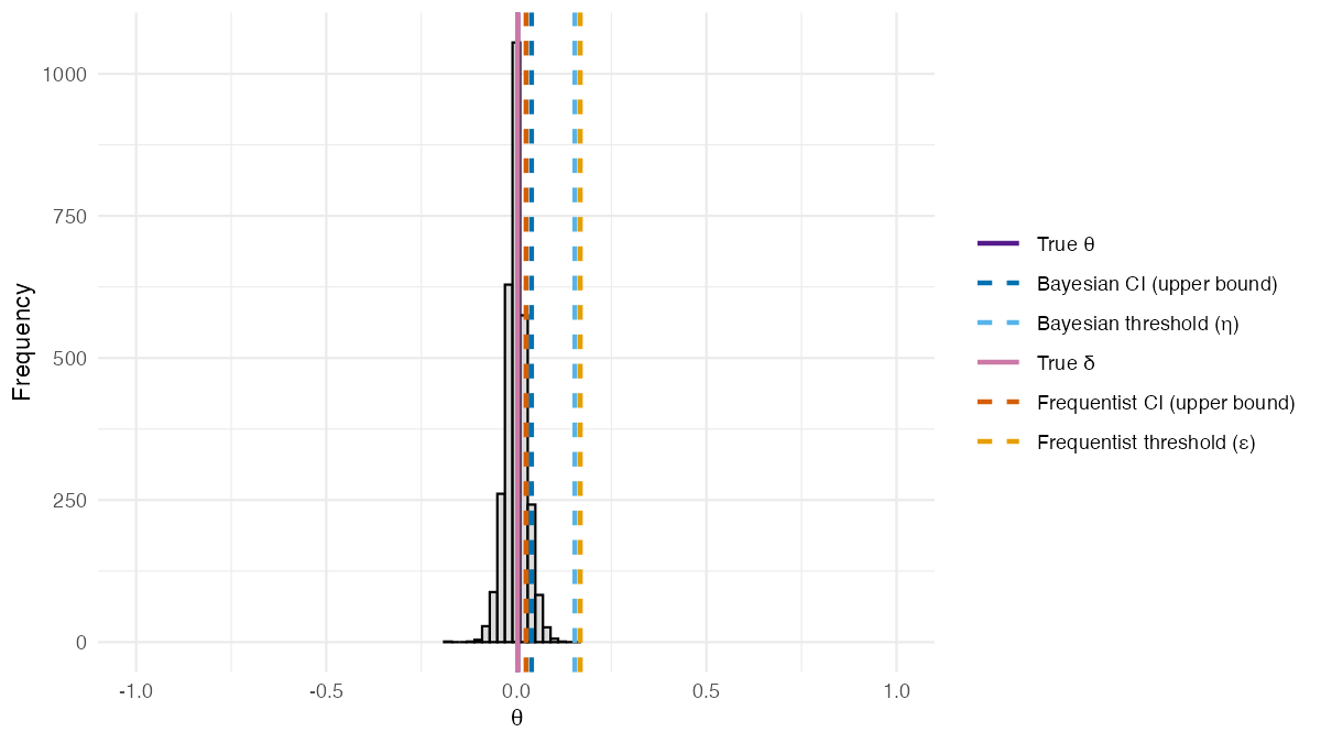
$Posterior distribution of $\theta$ from the BSET procedure without adjusting for covariates. Dashed lines show estimated quantities: the Bayesian 95\% credible interval upper bound and threshold $\eta$ (blue shades), and the frequentist 95\% confidence interval upper bound and threshold $\varepsilon$ (orange shades). Solid lines show the true values of $\theta$ (purple) and $\delta$ (pink).$

Posterior distribution of $\theta$ from the BSET procedure without adjusting for covariates. Dashed lines show estimated quantities: the Bayesian 95% credible interval upper bound and threshold $\eta$ (blue shades), and the frequentist 95% confidence interval upper bound and threshold $\varepsilon$ (orange shades). Solid lines show the true values of $\theta$ (purple) and $\delta$ (pink).

Two features of this result are worth highlighting. First, the posterior distribution of $\theta$ is centered around the true value of $\theta$ , demonstrating that the Bayesian imputation approach accurately recovers the true discrepancy between the treatment effects on $Y$ and $S$ . In this setting, covariates do not play a role in the data generating process, so the frequentist estimand $\delta$ coincides with $\theta$ and both methods perform similarly. Second, since the upper bound of the 95% credible interval falls below the validation threshold $\eta$ , the BSET procedure concludes that there is evidence that the surrogate is valid in this setting.

BSET with covariates

As an example, we can run the BSET procedure adjusting for covariates on the data generated from the first setting of Carlotti and Parast (2026). First of all, we need to prepare the data in the format required by BSET: a data frame with four columns, where the first column contains the observed values of the primary outcome $Y$ , the second column contains the observed values of the surrogate $S$ , the third column contains the treatment assignment $Z$ , and the fourth column contains the values of the binary covariate $X$ . We call $d$ the number of covariates, which in this case is equal to $2$ (including the intercept).

# Prepare the data for BSET (with covariates)
BSET_X_data <- data.frame(
  Y = data_X$P_observed[, "Y"],
  S = data_X$P_observed[, "S"],
  Z = data_X$Z,
  X = data_X$X
)

The posterior sampling parameters are defined in the same way as for the BSET procedure without adjusting for covariates. Whereas the prior parameters for the distribution of the potential outcomes in our Bayesian model are defined as follows:

mu_beta: A numeric vector of length $d$ containing the prior means for the regression coefficients of the potential outcomes on the covariates.
Sigma_beta: A numeric positive-definite matrix of dimension $d \times d$ containing the prior covariance matrix for the regression coefficients of the potential outcomes on the covariates.

# Prior parameters for the regression coefficients of the potential outcomes on the covariates
d <- 2
mu_beta <- rep(0, d)
Sigma_beta <- 10*diag(d)

We can also specify the true values of $\delta$ and $\theta$ as input to BSET to check if they are included in the posterior credible intervals. In this case, we can set $\delta$ and $\theta$ equal to the Monte Carlo estimates of $\delta$ and $\theta$ for setting 1 of Carlotti and Parast (2026).

Finally, we can run the BSET procedure adjusting for covariates as follows:

# Run the BSET procedure adjusting for covariates
BSET_X_results <- BSET::BSET(
  data = BSET_X_data,
  Y = "Y",
  S = "S",
  Z = "Z",
  X = "X",
  delta_true = estimands_Carlotti_and_Parast_2026$delta_MC[1],
  theta_true = estimands_Carlotti_and_Parast_2026$theta_MC[1],
  seed = 123,
  n_chains = n_chains,
  n_iter = n_iter,
  burn_in_ratio = burn_in_ratio,
  a = a,
  b = b,
  alpha = alpha,
  beta = beta,
  V_S_zero = V_S_zero,
  BF_alternative = BF_alternative,
  root_tolerance = 1e-16,
  mu_beta = mu_beta,
  Sigma_beta = Sigma_beta,
  s = s,
  tau = tau,
  plot = TRUE,
  mute = TRUE,
  parallel = TRUE
)

The posterior distribution of $\theta$ from the BSET procedure adjusting for covariates is shown in the figure below.

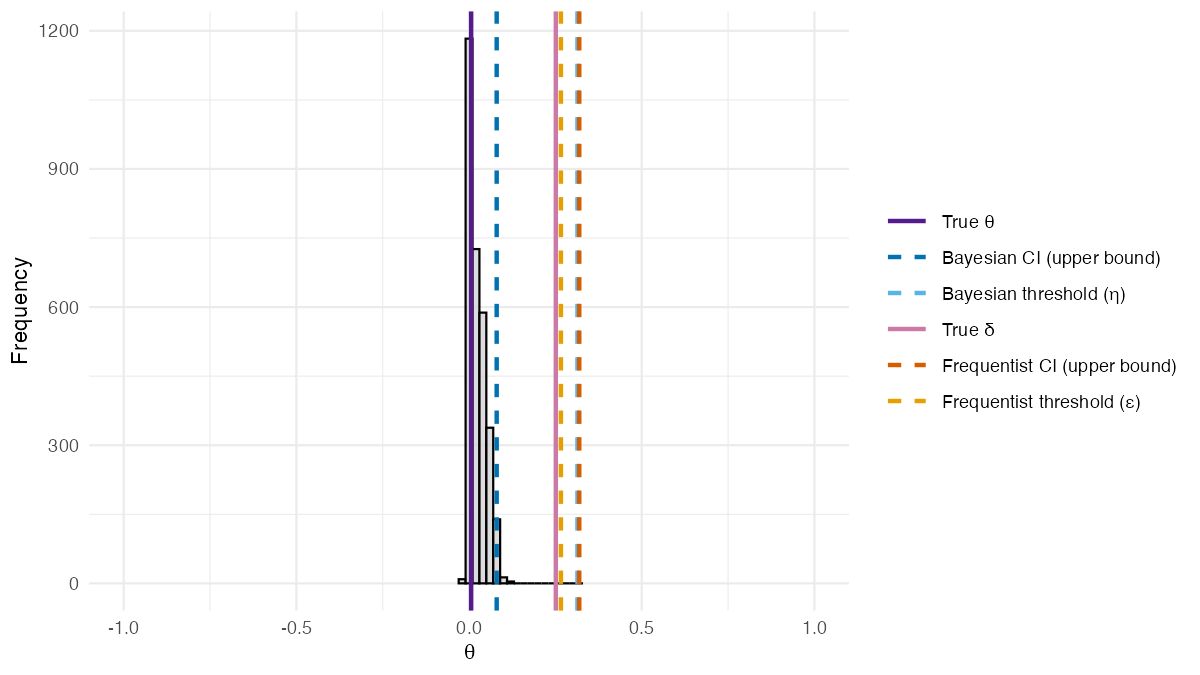
$Posterior distribution of $\theta$ from the BSET procedure adjusting for covariates. Dashed lines show estimated quantities: the Bayesian 95\% credible interval upper bound and threshold $\eta$ (blue shades), and the frequentist 95\% confidence interval upper bound and threshold $\varepsilon$ (orange shades). Solid lines show the true values of $\theta$ (purple) and $\delta$ (pink).$

Posterior distribution of $\theta$ from the BSET procedure adjusting for covariates. Dashed lines show estimated quantities: the Bayesian 95% credible interval upper bound and threshold $\eta$ (blue shades), and the frequentist 95% confidence interval upper bound and threshold $\varepsilon$ (orange shades). Solid lines show the true values of $\theta$ (purple) and $\delta$ (pink).

Unlike the previous setting, covariates now play a role in the data generating process, and this is where the two methods diverge. The posterior distribution of $\theta$ is still centered around its true value, confirming that the covariate-adjusted Bayesian model correctly recovers the true discrepancy parameter. In contrast, the frequentist estimand $\delta$ diverges substantially from the true $\theta$ , illustrating a key limitation of rank-based methods when covariates are present. Since the upper bound of the 95% credible interval falls below the validation threshold $\eta$ , the BSET procedure correctly concludes that there is evidence that the surrogate is valid in this setting, while the frequentist method, being based on $\delta$ , would incorrectly conclude that it is not.

References

Carlotti, Pietro, and Layla Parast. 2026. “A Bayesian Critique of Rank-Based Methods for Surrogate Marker Evaluation.” arXiv Preprint arXiv:2603.14381.

Parast, Layla, Tianxi Cai, and Lu Tian. 2024. “A Rank-Based Approach to Evaluate a Surrogate Marker in a Small Sample Setting.” Biometrics 80 (1): ujad035.

Pietro Carlotti

2026-05-04